ARIMA
learn learn~~
Page
Stationarity and differencing
A stationary time series is one whose statistical properties such as mean, variance, autocorrelation, etc. are all constant over time. Most statistical forecasting methods are based on the assumption that the time series can be rendered approximately stationary (i.e., “stationarized”) through the use of mathematical transformations. A stationarized series is relatively easy to predict: you simply predict that its statistical properties will be the same in the future as they have been in the past! (Recall our famous forecasting quotes.) The predictions for the stationarized series can then be “untransformed,” by reversing whatever mathematical transformations were previously used, to obtain predictions for the original series. (The details are normally taken care of by your software.) Thus, finding the sequence of transformations needed to stationarize a time series often provides important clues in the search for an appropriate forecasting model. Stationarizing a time series through differencing (where needed) is an important part of the process of fitting an ARIMA model, as discussed in the ARIMA pages of these notes.
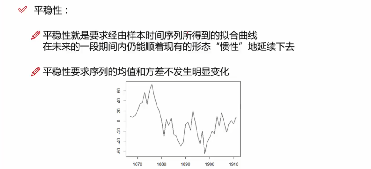

基本都是若平稳 严平稳不太现实
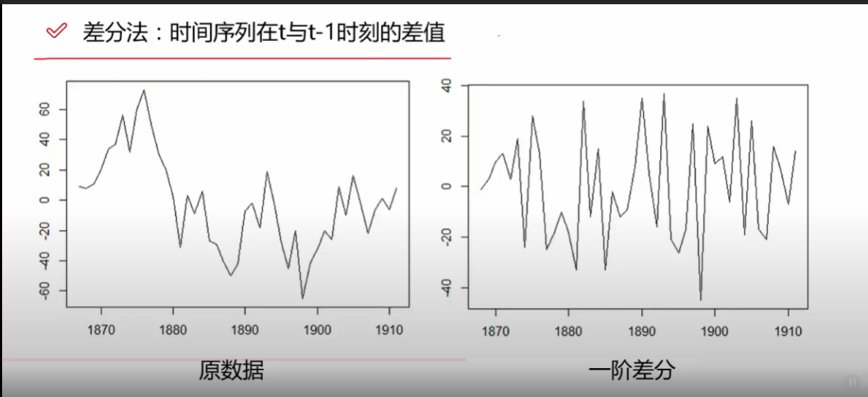
差分法可以使得数据变得更加平稳
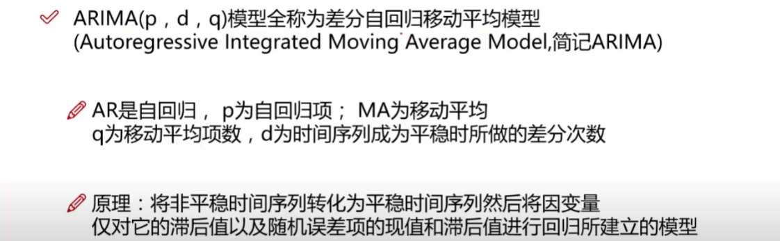
What does the p, d and q in ARIMA model mean
the value of d, therefore, is the minimum number of differencing needed to make the series stationary. And if the time series is already stationary, then d = 0.
p is the order of the ‘Auto Regressive’ (AR) term. It refers to the number of lags of Y to be used as predictors. And q is the order of the ‘Moving Average’ (MA) term. It refers to the number of lagged forecast errors that should go into the ARIMA Model.
you can understand more clearly by reading next chapter
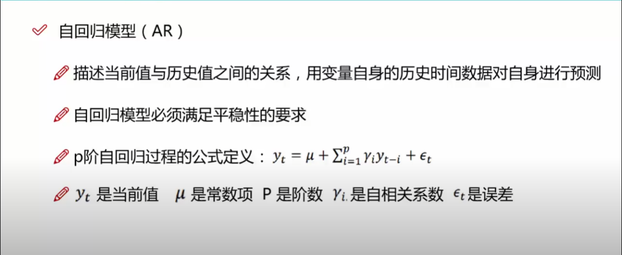
What are AR and MA models
AR
限制

MA

AR+MA

ARIMA
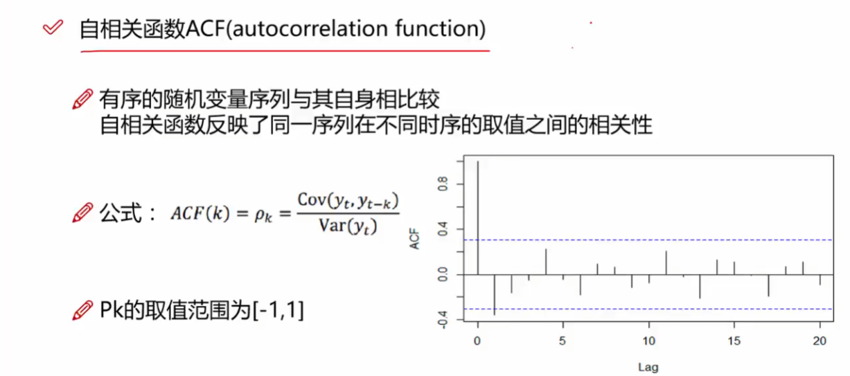
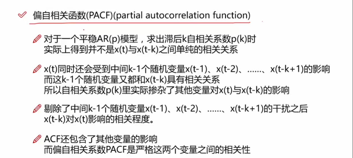
what is ACF and PACF
ACF
PACF
单纯地考虑 x(t) 和 x(t-k) 的关系
https://timeseriesreasoning.com/contents/partial-auto-correlation/
https://online.stat.psu.edu/stat510/lesson/2/2.2
How to find the order of the MA term (p,q,d)
How to find the order of differencing (d) in ARIMA model
The purpose of differencing it to make the time series stationary.
But you need to be careful to not over-difference the series. Because, an over differenced series may still be stationary, which in turn will affect the model parameters.
The right order of differencing is the minimum differencing required to get a near-stationary series which roams around a defined mean and the ACF plot reaches to zero fairly quick.
If the autocorrelations are positive for many number of lags (10 or more), then the series needs further differencing. On the other hand, if the lag 1 autocorrelation itself is too negative, then the series is probably over-differenced.
In the event, you can’t really decide between two orders of differencing, then go with the order that gives the least standard deviation in the differenced series.
check if the series is stationary using the Augmented Dickey Fuller test (adfuller()), from the statsmodels package.
1 | import numpy as np, pandas as pd |
(*)
1 | from statsmodels.tsa.stattools import adfuller |
we got
1 | ADF Statistic: -2.464240 |
if P Value > 0.05 we go ahead with finding the order of differencing.
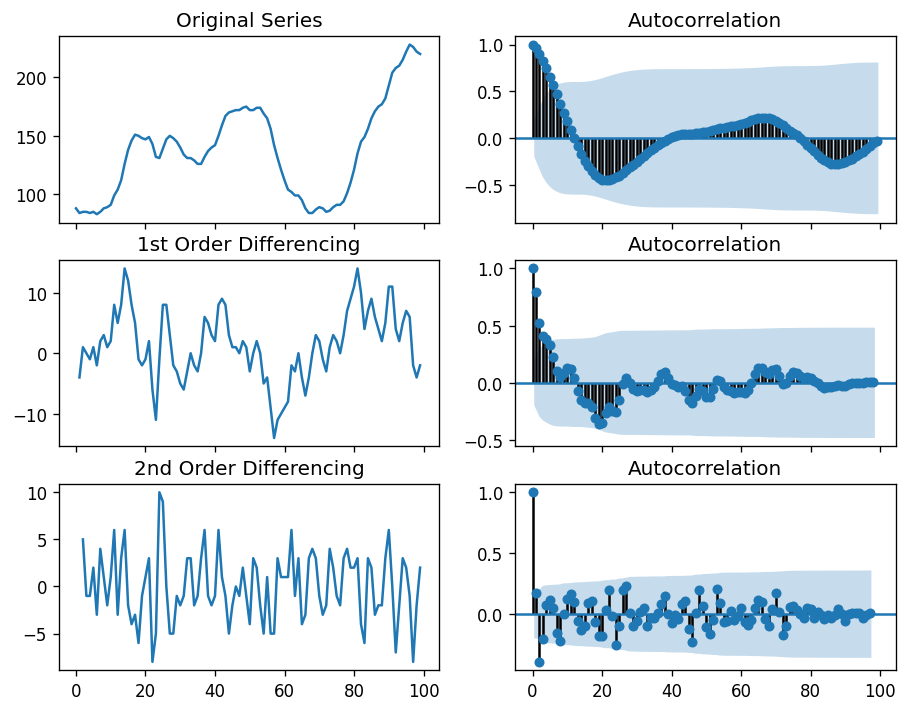
Since P-value is greater than the significance level, we difference the series. please look at picture (*).
For the above series, the time series reaches stationarity with two orders of differencing. But on looking at the autocorrelation plot for the 2nd differencing the lag goes into the far negative zone fairly quick, which indicates, the series might have been over differenced.
So, I am going to tentatively fix the order of differencing as 1 even though the series is not perfectly stationary (weak stationarity).
1 | import pandas as pd |
ndiffs的文档–Number of differences required for a stationary series
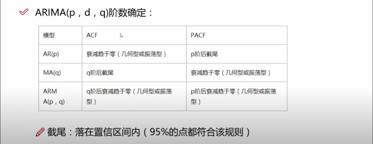
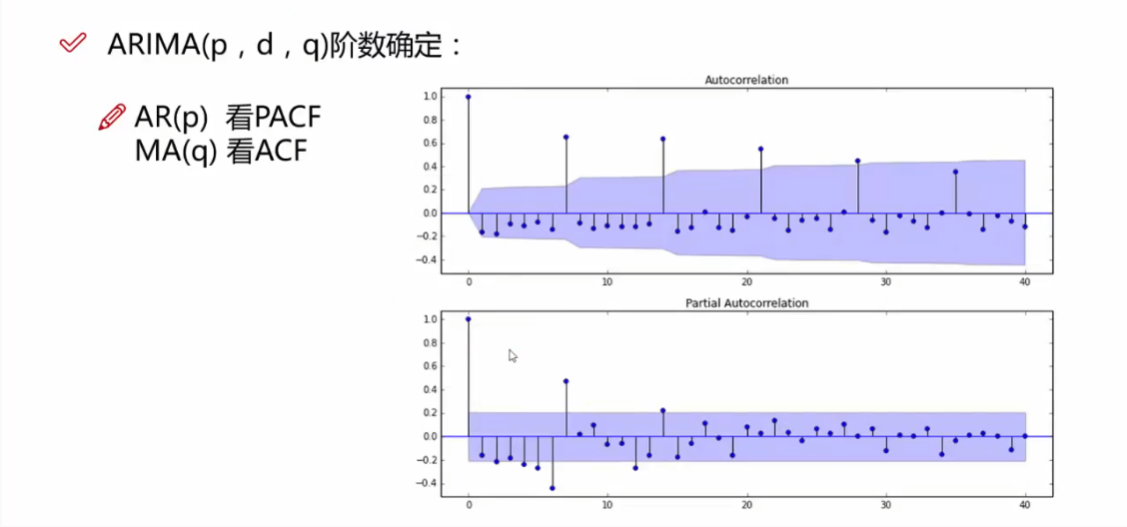
How to find the order of the AR term (p)
How to find the order of the MA term (q)
(1)ACF和PACF 利用拖尾和截尾来确定(这里还是有点没太完全清楚,,,感觉我的判断和网上说的有点区别。。。反正代码可以自动找。。。)
(2)信息准则定阶(AIC、BIC、HQIC)
How to build the ARIMA Model

1 | import numpy as np, pandas as pd |
result:
1 | ARIMA Model Results |
The model summary reveals a lot of information. The table in the middle is the coefficients table where the values under ‘coef’ are the weights of the respective terms.
Notice here the coefficient of the MA2 term is close to zero and the P-Value in ‘P>|z|’ column is highly insignificant. It should ideally be less than 0.05 for the respective X to be significant.
So, let’s rebuild the model without the MA2 term.
1 | # 1,1,1 ARIMA Model |
result
1 | ARIMA Model Results |
The model AIC has reduced, which is good. The P Values of the AR1 and MA1 terms have improved and are highly significant (<< 0.05).
Let’s plot the residuals to ensure there are no patterns (that is, look for constant mean and variance).
1 | residuals = pd.DataFrame(model_fit.resid) |
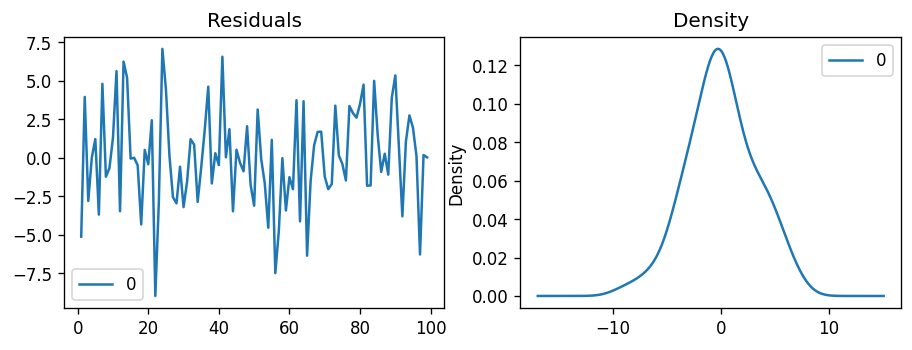
The residual errors seem fine with near zero mean and uniform variance. Let’s plot the actuals against the fitted values using plot_predict().
1 | # Actual vs Fitted |
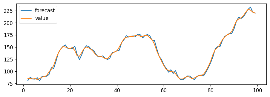
When you set dynamic=False the in-sample lagged values are used for prediction.
That is, the model gets trained up until the previous value to make the next prediction. This can make the fitted forecast and actuals look artificially good.
So, we seem to have a decent ARIMA model. But is that the best?
Can’t say that at this point because we haven’t actually forecasted into the future and compared the forecast with the actual performance.
So, the real validation you need now is the Out-of-Time cross-validation.
How to do find the optimal ARIMA model manually using Out-of-Time Cross validation
In Out-of-Time cross-validation, you take few steps back in time and forecast into the future to as many steps you took back. Then you compare the forecast against the actuals.
To do out-of-time cross-validation, you need to create the training and testing dataset by splitting the time series into 2 contiguous parts in approximately 75:25 ratio or a reasonable proportion based on time frequency of series.
Why am I not sampling the training data randomly you ask?
That’s because the order sequence of the time series should be intact in order to use it for forecasting.
1 | from statsmodels.tsa.stattools import acf |
we can now build the ARIMA model on training dataset, forecast and plot it.
1 | # Build Model |
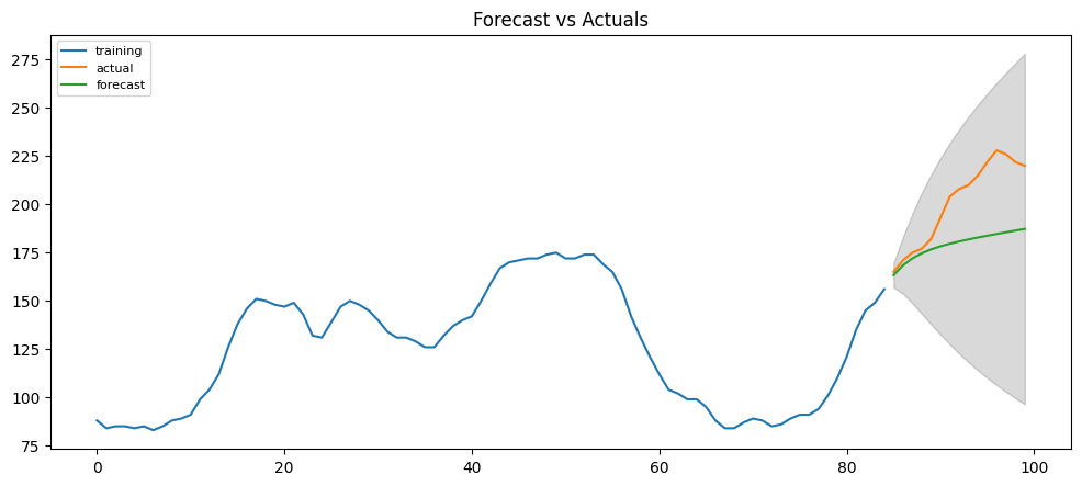
From the chart, the ARIMA(1,1,1) model seems to give a directionally correct forecast. And the actual observed values lie within the 95% confidence band. That seems fine.
But each of the predicted forecasts is consistently below the actuals. That means, by adding a small constant to our forecast, the accuracy will certainly improve. So, there is definitely scope for improvement.
So, what I am going to do is to increase the order of differencing to two, that is set d=2 and iteratively increase p to up to 5 and then q up to 5 to see which model gives least AIC and also look for a chart that gives closer actuals and forecasts.
While doing this, I keep an eye on the P values of the AR and MA terms in the model summary. They should be as close to zero, ideally, less than 0.05.
1 | # Build Model |
1 | ARIMA Model Results |
The AIC has reduced to 440 from 515. Good. The P-values of the X terms are less the < 0.05, which is great.
So overall it’s much better.
Ideally, you should go back multiple points in time, like, go back 1, 2, 3 and 4 quarters and see how your forecasts are performing at various points in the year.
Here’s a great practice exercise: Try to go back 27, 30, 33, 36 data points and see how the forcasts performs. The forecast performance can be judged using various accuracy metrics discussed next.
Accuracy Metrics for Time Series Forecast
The commonly used accuracy metrics to judge forecasts are:
- Mean Absolute Percentage Error (MAPE)
- Mean Error (ME)
- Mean Absolute Error (MAE)
- Mean Percentage Error (MPE)
- Root Mean Squared Error (RMSE)
- Lag 1 Autocorrelation of Error (ACF1)
- Correlation between the Actual and the Forecast (corr)
- Min-Max Error (minmax)
Typically, if you are comparing forecasts of two different series, the MAPE, Correlation and Min-Max Error can be used.
Why not use the other metrics?
Because only the above three are percentage errors that vary between 0 and 1. That way, you can judge how good is the forecast irrespective of the scale of the series.
The other error metrics are quantities. That implies, an RMSE of 100 for a series whose mean is in 1000’s is better than an RMSE of 5 for series in 10’s. So, you can’t really use them to compare the forecasts of two different scaled time series.
1 | # Accuracy metrics |
Around 2.2% MAPE implies the model is about 97.8% accurate in predicting the next 15 observations.
Now you know how to build an ARIMA model manually.
But in industrial situations, you will be given a lot of time series to be forecasted and the forecasting exercise be repeated regularly.
So we need a way to automate the best model selection process.
How to do Auto Arima Forecast in Python
Like R’s popular auto.arima() function, the pmdarima package provides auto_arima() with similar functionality.
auto_arima() uses a stepwise approach to search multiple combinations of p,d,q parameters and chooses the best model that has the least AIC.
1 | from statsmodels.tsa.arima_model import ARIMA |
1 | Performing stepwise search to minimize aic |
I met a bug here
1 | ARIMA(3,2,1)(0,0,0)[0] intercept : AIC=inf, Time=1.25 sec |
why AIC == inf ?
How to build SARIMAX Model with exogenous variable
https://raw.githubusercontent.com/selva86/datasets/master/a10.csv
1 | # Import Data |
1 | # Compute Seasonal Index |
1 | import pmdarima as pm |
https://zhuanlan.zhihu.com/p/157960700
https://analyticsindiamag.com/complete-guide-to-sarimax-in-python-for-time-series-modeling/
bug
tips
parameter
https://alkaline-ml.com/pmdarima/tips_and_tricks.html
How to decide m?
In my code, maybe I need to set m = 7.
- 7 - daily
- 12 - monthly
- 52 - weekly
let’s take a look at one question
I have two large time series data. One is separated by seconds intervals and the other by minutes. The length of each time series is 180 days. I’m using R (3.1.1) for forecasting the data. I’d like to know the value of the “frequency” argument in the ts() function in R, for each data set. Since most of the examples and cases I’ve seen so far are for months or days at the most, it is quite confusing for me when dealing with equally separated seconds or minutes. According to my understanding, the “frequency” argument is the number of observations per season. So what is the “season” in the case of seconds/minutes? My guess is that since there are 86,400 seconds and 1440 minutes a day, these should be the values for the “freq” argument. Is that correct?
Yes, the “frequency”is the number of observations per “cycle” (normally a year, but sometimes a week, a day or an hour). This is the opposite of the definition of frequency in physics, or in Fourier analysis, where “period” is the length of the cycle, and “frequency” is the inverse of period. When using the ts() function in R, the following choices should be used.
| Data | Frequency |
|---|---|
| Annual | 1 |
| Quarterly | 4 |
| Monthly | 12 |
| Weekly | 52 |
Actually, there are not 52 weeks in a year, but 365.25/7 = 52.18 on average, allowing for a leap year every fourth year. But most functions which use ts objects require integer frequency.
If the frequency of observations is greater than once per week, then there is usually more than one way of handling the frequency. For example, data with daily observations might have a weekly seasonality (frequency=7) or an annual seasonality (frequency=365.25). Similarly, data that are observed every minute might have an hourly seasonality (frequency=60), a daily seasonality (frequency=24x60=1440), a weekly seasonality (frequency=24x60x7=10080) and an annual seasonality (frequency=24x60x365.25=525960). If you want to use a ts object, then you need to decide which of these is the most important.
An alternative is to use a msts object (defined in the forecast package) which handles multiple seasonality time series. Then you can specify all the frequencies that might be relevant. It is also flexible enough to handle non-integer frequencies.
| Frequencies | |||||
|---|---|---|---|---|---|
| Data | Minute | Hour | Day | Week | Year |
| Daily | 7 | 365.25 | |||
| Hourly | 24 | 168 | 8766 | ||
| Half-hourly | 48 | 336 | 17532 | ||
| Minutes | 60 | 1440 | 10080 | 525960 | |
| Seconds | 60 | 3600 | 86400 | 604800 | 31557600 |
You won’t necessarily want to include all of these frequencies — just the ones that are likely to be present in the data. For example, any natural phenomena (e.g., sunshine hours) is unlikely to have a weekly period, and if your data are measured in one-minute intervals over a 3 month period, there is no point including an annual frequency.
For example, the taylor data set from the forecast package contains half-hourly electricity demand data from England and Wales over about 3 months in 2000. It was defined as
1 | taylor <- msts(x, seasonal.periods=c(48,336) |
One convenient model for multiple seasonal time series is a TBATS model:
1 | taylor.fit <- tbats(taylor) |
(Warning: this takes a few minutes.)
If an msts object is used with a function designed for ts objects, the largest seasonal period is used as the “frequency” attribute.
Some ideas and questions?
- The ARIMA model seems to process good result for short-term forecasting, but it is difficult to get results in the long-term prediction. So it seems unconvincing to use the ARIMA model as a comparative experiment in long-term forecasting?
- In my experiments, I found that a more accurate setting of the seasonal(parameter m) resulted in increased training time and made it difficult for my experiments to continue.
reference
https://otexts.com/fpp2/stationarity.html
https://people.duke.edu/~rnau/411home.htm
https://www.machinelearningplus.com/time-series/arima-model-time-series-forecasting-python/
https://www.youtube.com/watch?v=ikkOBWQj9X8
https://www.machinelearningplus.com/time-series/augmented-dickey-fuller-test/
https://robjhyndman.com/hyndsight/seasonal-periods/
https://alkaline-ml.com/pmdarima/modules/generated/pmdarima.arima.auto_arima.html