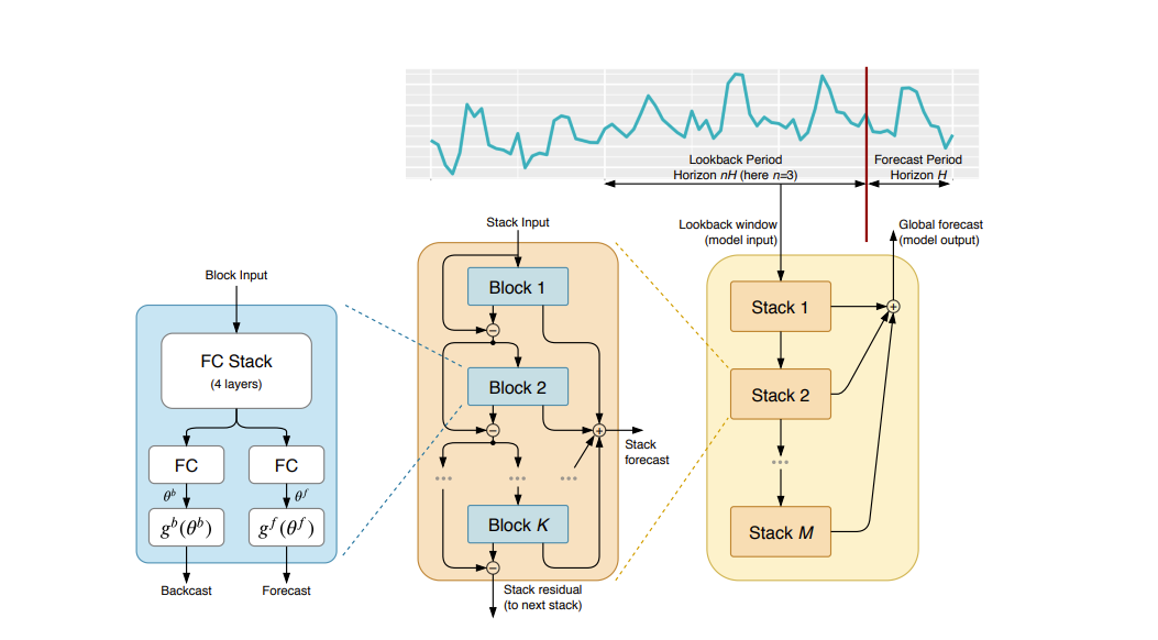
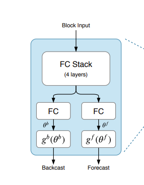
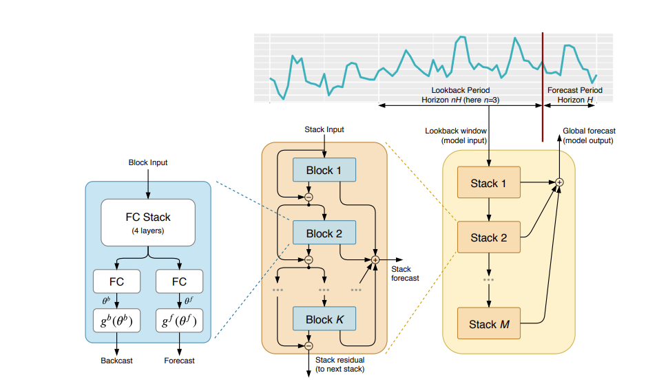
N-BEATS model is based on backward and forward residual links and a very deep stack of fully-connected layers. Our architecture design methodology relies on a few key principles. First, the base architecture should be simple and generic, yet expressive (deep). Second, the architecture should not rely on timeseries-specific feature engineering or input scaling. These prerequisites let us explore the potential of pure DL architecture in TS horizoning. Finally, as a prerequisite to explore interpretability, the architecture should be extendable towards making its outputs human interpretable. We now discuss how those principles converge to the proposed architecture.
一开头 就让我十分感动 作者提出了两点
First, the base architecture should be simple and generic, yet expressive (deep).
Second, the architecture should not rely on timeseries-specific feature engineering or input scaling
# This Python 3 environment comes with many helpful analytics libraries installed
# It is defined by the kaggle/python Docker image: https://github.com/kaggle/docker-python
# For example, here's several helpful packages to load

import numpy as np # linear algebra
import pandas as pd # data processing, CSV file I/O (e.g. pd.read_csv)
from sklearn.metrics import median_absolute_error
import random
import datetime

import tensorflow as tf
from tensorflow import keras
from tensorflow.python.keras.losses import LossFunctionWrapper
from tensorflow.python.keras.utils import losses_utils
import tensorflow_probability as tfp
from tensorflow.keras.callbacks import ReduceLROnPlateau, EarlyStopping
tfd = tfp.distributions

import matplotlib.pyplot as plt
import plotly.graph_objects as go
from plotly.subplots import make_subplots
import plotly.express as px

!pip install -q -U keras-tuner

import keras_tuner as kt
import IPython

# Input data files are available in the read-only "../input/" directory
# For example, running this (by clicking run or pressing Shift+Enter) will list all files under the input directory

import os
for dirname, _, filenames in os.walk('/kaggle/input'):
    for filename in filenames:
        print(os.path.join(dirname, filename))

# You can write up to 20GB to the current directory (/kaggle/working/) that gets preserved as output when you create a version using "Save & Run All"
# You can also write temporary files to /kaggle/temp/, but they won't be saved outside of the current session
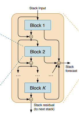
classStack(tf.keras.layers.Layer): """A stack is a series of blocks where each block produce two outputs, the horizon and the back_horizon. All of the outputs are sum up which compose the stack output while each residual back_horizon is given to the following block. Parameters ---------- blocks: list of `TrendBlock`, `SeasonalityBlock` or `GenericBlock`. Define blocks in a stack. """ def__init__(self, blocks, **kwargs): super().__init__(**kwargs)
classN_BEATS(tf.keras.Model): """This class compute the N-BEATS model. This is a univariate model which can be interpretable or generic. It's strong advantage is its internal structure which allows us to extract the trend and the seasonality of a temporal serie. It's available from the attributes `seasonality` and `trend`. This is an unofficial implementation. `@inproceedings{ Oreshkin2020:N-BEATS, title={{N-BEATS}: Neural basis expansion analysis for interpretable time series horizoning}, author={Boris N. Oreshkin and Dmitri Carpov and Nicolas Chapados and Yoshua Bengio}, booktitle={International Conference on Learning Representations}, year={2020}, url={https://openreview.net/forum?id=r1ecqn4YwB} }` Parameter --------- stacks: list of `Stack` layer. Define the stack to use in nbeats model. It can be full of `TrendBlock`, `SeasonalityBlock` or `GenereicBlock`. """ def__init__(self, stacks, **kwargs): super().__init__(**kwargs)
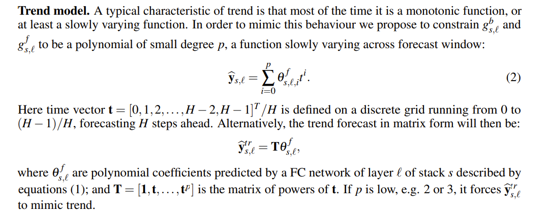
classTrendBlock(tf.keras.layers.Layer): """ Trend block definition. Output layers are constrained which define polynomial function of small degree p. Therefore it is possible to get explanation from this block. Parameter --------- p_degree: integer Degree of the polynomial function. horizon: integer Horizon time to horizon. back_horizon: integer Past to rebuild. n_neurons: integer Number of neurons in Fully connected layers. n_quantiles: Integer. Number of quantiles in `QuantileLossError`. """ def__init__(self, horizon, back_horizon, p_degree, n_neurons, n_quantiles, dropout_rate, **kwargs):
super().__init__(**kwargs) self._p_degree = tf.reshape(tf.range(p_degree + 1, dtype='float32'), shape=(-1, 1)) # Shape (-1, 1) in order to broadcast horizon to all p degrees self._horizon = tf.cast(horizon, dtype='float32') self._back_horizon = tf.cast(back_horizon, dtype='float32') self._n_neurons = n_neurons self._n_quantiles = n_quantiles
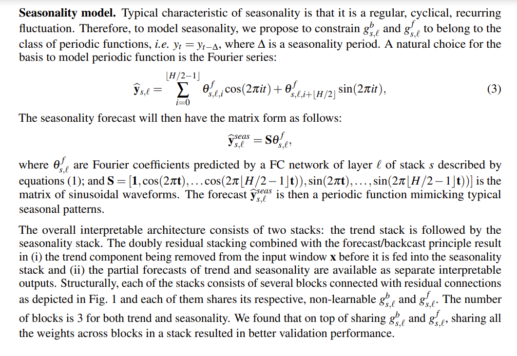
classSeasonalityBlock(tf.keras.layers.Layer): """Seasonality block definition. Output layers are constrained which define fourier series. Each expansion coefficent then become a coefficient of the fourier serie. As each block and each stack outputs are sum up, we decided to introduce fourier order and multiple seasonality periods. Therefore it is possible to get explanation from this block. Parameters ---------- horizon: integer Horizon time to horizon. back_horizon: integer Past to rebuild. n_neurons: integer Number of neurons in Fully connected layers. periods: Integer. fourier serie period. The paper set this parameter to `horizon/2`. back_periods: Integer. fourier serie back period. The paper set this parameter to `back_horizon/2`. horizon_fourier_order: Integer. Higher values signifies complex fourier serie back_horizon_fourier_order: Integer. Higher values signifies complex fourier serie n_quantiles: Integer. Number of quantiles in `QuantileLossError`. """ def__init__(self, horizon, back_horizon, n_neurons, periods, back_periods, horizon_fourier_order, back_horizon_fourier_order, n_quantiles, dropout_rate, **kwargs): super().__init__(**kwargs)
self._horizon = horizon self._back_horizon = back_horizon self._periods = tf.cast(tf.reshape(periods, (1, -1)), 'float32') # Broadcast horizon on multiple periods self._back_periods = tf.cast(tf.reshape(back_periods, (1, -1)), 'float32') # Broadcast back horizon on multiple periods self._horizon_fourier_order = tf.reshape(tf.range(horizon_fourier_order, dtype='float32'), shape=(-1, 1)) # Broadcast horizon on multiple fourier order self._back_horizon_fourier_order = tf.reshape(tf.range(back_horizon_fourier_order, dtype='float32'), shape=(-1, 1)) # Broadcast horizon on multiple fourier order
# Workout the number of neurons needed to compute seasonality coefficients horizon_neurons = tf.reduce_sum(2 * horizon_fourier_order) back_horizon_neurons = tf.reduce_sum(2 * back_horizon_fourier_order) self._FC_stack = [tf.keras.layers.Dense(n_neurons, activation='relu', kernel_initializer="glorot_uniform") for _ inrange(4)] self._dropout = tf.keras.layers.Dropout(dropout_rate) self._FC_back_horizon = self.add_weight(shape=(n_neurons, back_horizon_neurons), trainable=True, initializer="glorot_uniform", name='FC_back_horizon_seasonality')
for dense in self._FC_stack: inputs = dense(inputs) # shape: (Batch_size, nb_neurons) inputs = self._dropout(inputs, training=True) # We bind first layers by a dropout